Introduction

Lindenmeyer Systems or L-Systems have proven to be one of the most popular methods for populating computer-generated scenes with plant-like objects. Yet, as is easily seen in the natural world, the amount of data produced from L-Systems can be enormous. The goal of the Branching Shadows project was to integrate an L-System generator (often called an L-Parser) into a ray-tracer so that some of this data is generated at render-time. Doing this in an efficient way was one of the unique challenges of this project. This document details the results and outlines areas of future work.

Background

This project dealt with only the simplest of L-Systems—non-random, context-free, and lacking in any symbolic conditions or expressions. These L-Systems consist of a set of "productions" which each have a name and a corresponding "successor". The successor is a list of symbols which either identify another production or a command to be interpreted by the L-Parser. An L-Parser then takes an initial successor and substitutes production symbols with their successors and then reiterates this process for a user-defined number of times.

Trees and plants are then generated by interpreting the final list of symbols as commands which direct a "turtle" (as in the old turtle graphics). A turtle 'state' consists of a coordinate system with a 'forward', 'left', and 'up' vector; a branch length; a branch thickness; and an angle which is used for rotating the coordinate system. For details about how these symbols manipulate the turtle state variables, see the Turtle Commands. For a more a more comprehensive summary of L-Systems, see the Project Proposal.

Basic Algorithm Overview

The general idea behind this algorithm is to generate some or all of the L-System geometry every time a ray intersection test is executed. This is done efficiently by enclosing each L-System branch in a bounding shape which is tested before traversing deeper into the tree heirarchy. So if one views a tree as a series of connected segments (an axis) with any number of bounded branches diverging from that axis (each of which is itself an axis), then an intersection algorithm would only need to test each segment (cylinders in this project) in the axis and then recursively test each branch whose bounding shape is hit. (For more details about axial trees, see reference [2] p. 21.) So long as a sufficient number of branches are 'pruned', the high-cost of generating/interpreting the L-System is avoided.

Here is a very simple pseudo-code intersection routine that illustrates this concept:

LSystemIntersect (ray r, real &t) {
    real tempT;
    Foreach axial segment S { 
        Construct a cylinder C from S
        C.CylinderIntersect(r, tempT);
        If (tempT < t)  
            t = tempT;  
    }
    Foreach branch B { 
        If (B.BoundIntersect(r)) { 
            B.LSystemIntersect(r, tempT);
            If (tempT < t)
                t = tempT; 
        } 
    }
}

The tricky part of this algorithm is the way the bounding shapes correspond to the underlying L-System and deciding how much of the L-System generation and interpretation is done at render-time.

Algorithm Details

Initial L-System Representation

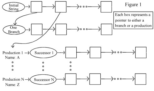
The initial L-System representation (before substitutions) is depicted in Figure 1. Each production has a name and a pointer to a successor. A successor contains a list of elements (which I shall call nodes) which can point to either another successor (which represents a branch) or a production (which represents a symbol). Any production that has no successor nodes (i.e. the symbol F stands for nothing but a turtle command) points to an empty successor. Another list, not shown, keeps track of all the productions and a successor pointer indicates the root of the entire tree.

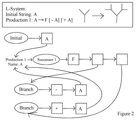
Figure 2 shows an example.

Parsing

In this project, parsing is done using Flex and Bison and takes in an input file like the following:

iterations 10
angle 10
length 1
thickness 1
startpoint 0 0 0
forward 0 0 1
left 1 0 0<
up 0 1 0
F F F F F F F F F F >(1) &(1) A
A --> !(.75) t(.4) F B >(94) B >(132) B
B --> [ & " t(.4) !(.75) F L [ +(180) F L ] $ A L [ +(180) F L ] ]
L --> [ F +(180) { +(30) F -(120) F -(120) F } ]

See the commands for details about what each symbol does.

During parsing a symbol table is maintained so that production symbols appearing before the production is defined can still be correctly used. Production names can be full strings and must be generally seperated by spaces.

L-System Generation

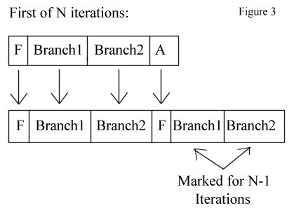
The actual generation of the L-System, complete with substitutions, is done using arrays of nodes—each of which can point to either a branch or a production. For a single iteration of a successor object, two arrays are used—one that contains the source successor (copied over from the initial representation) and one for the expanded successor. We then loop through all of the nodes in the source. If the node points to an empty production or it points to a branch (branches are not expanded here) then the node is copied directly to the destination. Otherwise, the node points to a production whose nodes are then copied over.

To iterate a successor N times, this process is repeated N times by switching the source and destination buffer in between each pass. Also, in order to correctly iterate branches in subsequent recursive calls, each branch brought in through a substitution must be marked with the number of iterations that should be done on it—so that if we were substituting a branch on the first of N iterations, it would be marked with N-1. See Figure 3 for an example based on the L-System in Figure 2.

Bounding Cubes

My solution to the bounding shape problem was to associate an oriented bounding cube with each [branchID, # of iterations] pair and to make the cube's dimensions relative to the length variable in the turtle state. This way the bounding shape is valid no matter what state the turtle is in. Each branch (including the initial list of symbols) is given an identification number which, along with the number of iterations to expand that branch, indexes into a two dimensional array which contains the relative bounding cube. So if the initial successor had an ID 0, then the bounding cube for that single successor would be [0, 0], and if the L-System was being expanded with N iterations, the entire tree bounding cube would be indexed by [0, N].

The dimensions of these bounding cubes are determined in a preprocessing stage which iterates over the entire L-System. When a successor is generated for a given number of iterations, each axial segment is incorporated into the dimensions of the corresponding cube. Also, the cube is added to a list and passed recursively to all subsequent branches—which then incorporate their segments into all parent bounding cubes. Another way to do this would be for the recursive call to return the branches' cube and have the parent incorporate it into their own. This, however, leads to an unecessary enlargement of the parent cube since the cube's corners may easily protrude further than the segments themselves.

Another speedup using bounding cubes is to bound the axis segments as well all of the branches.

The Cache

Instead of generating the L-System for each axis everytime an intersection occurs, a cache is used to store already generated buffers. The cache consists of a list of buffers that can be used for generation. The 2D array mentioned in the previous section is also used to indicate whether a given [branchID, # of iterations] buffer is in the cache. If it is, it is used directly and not generated. If not, a buffer is replaced using a least-recently-used policy.

There is an added complication that occurs when using the recursive intersection tests—if a parent axis generates a buffer and expects it to be around after a recursive call, the buffer must be locked so that it cannot be replaced. Because of this, enough buffers must be allocated to account for the deepest recursive call. Of course it is also possible to work around this by doing the recursive calls after all of the axis segments have been processed.

Preprocessing

In my implementation there are two preprocessing stages. Both of them iterate through the entire L-System but perform different tasks. The first is used mainly for counting certain properties of the L-System, such as the maximum length of any iterated successor list and how many limbs occur in a given [branchID, # of iterations] pair. This information is then used to optimize the size of the generation buffers and the size of the cache. The second proprocessing stage calculates all of the bounding cube information.

Intersection Routine

The intersection routine is essentially the same as the generic pseudo-code listed in the overview but with some of the L-System and cache details added in. Here is a more detailed version:

LSystemIntersect (ray r, real &t, int iterations) {
    real tempT; 
    String symbolName; 
    treeBound bound;

    treeBuffer generatedBuffer = Cache.RequestBuffer(myID, iterations);

    If (generatedBuffer is empty) { 
        generatedBuffer = Cache.RequestNewBuffer(myID, iterations); 
        generatedBuffer = GenerateBuffer(myID, iterations); 
    }

    Foreach symbol S in generatedBuffer { 
        if (S.isBranch()) { 
            bound = getBound(S.getID(), S.getIterations()); 
            If (bound.intersect(r)) { 
                B.LSystemIntersect(r, tempT);
                If (tempT < t) 
                    t = tempT; 
            } 
        } else { 
            symbolName = S.getProduction().getName();

            if (symbolName == "F") {
                Move Turtle in Turtle's forward direction 

                Construct a cylinder C from the old point and the new point and the current thickness 
                C.CylinderIntersect(r, tempT);

                If (tempT < t) 
                    t = tempT; 
            } else 
                evaluateSymbol(symbolName) 
        } 
    } 
}

Sorting The Intersection Depths

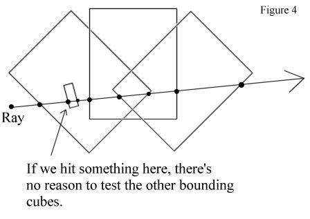
Another speedup that can be added to the intersect routine is to keep track of the intersection depth of the bounding cubes. These depths and their corresponding branches are then sorted so that we recursively call them in the order of their depth (closest first). If we already have an intersection (either from a branch or from an axis segment) that is closer than the depth of the the bounding cube then we can stop. Figure 4 illustrates this idea.

This speedup proved highly effective in densly populated L-Systems. (See the Graphs section.)

Results

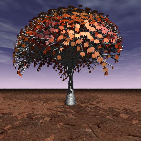
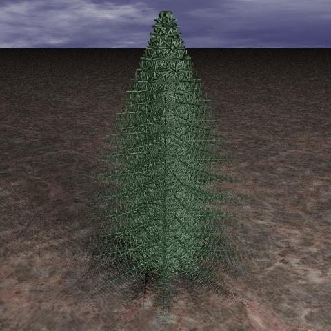
Images

Graphs And Samples

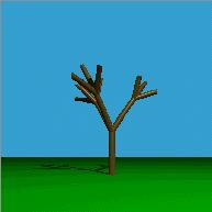
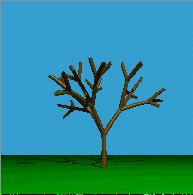
Sample A

Input File:

angle 30
thickness .20
length 1
startpoint 0 0 0
forward 0 0 1
left 1 0 0
up 0 1 0

FP A

A --> !(.9) t(.1) FP B >(94) B >(132) B
B --> [ & t(.1) FP $ A ]
FP --> '(1.25) F '(.8)

Sample Images:

(Don't ask why some of the upper branches are green — some defect in my ray-tracer.)
 

5 Iterations	7 Iterations	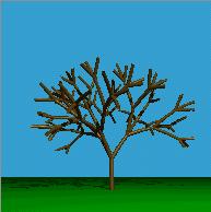9 Iterations
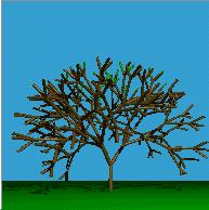11 Iterations	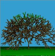13 Iterations	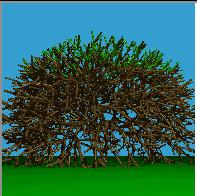15 Iterations
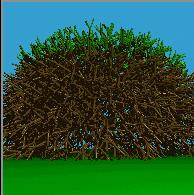17 Iterations	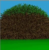19 Iterations

Graphs:

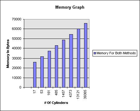
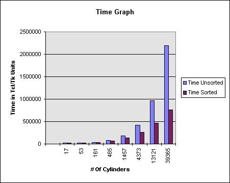
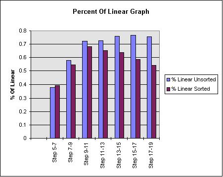
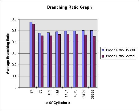
The following graphs compare the performance of two versions of the algorithm. The unsorted version will always recurse down a child branch if that branch's bounding cube is hit. The sorted version sorts the intersection depth of the bounding cubes and will stop recursing once an intersection point is found that is closer than the start of the next cube. See the Sorting section above.

This next graph displays how the method compares with linear performance. The ratio going from step N to N+1 is calculated in the following way:

% Linear = (Time(N+1) / Time(N)) / (Cylinders(N+1) / Cylinders(N))

So that if we doubled the amount of cylinders and our time also doubled, we would have a ratio of 1—the expected performance of a linear algorithm.

The next graph illustrates the average percentage of child branches being traversed based on the bounding box tests. In effect, this is the only difference between the sorted and unsorted methods — one produces a lower ratio. A difference of 3-5 % is responsible for the major speed improvements shown in the time graph.

Future Work

There are many possible areas for future work. One obvious area is to expand the breadth of L-Systems which the algorithm can effectively handle—though the problems created by more complex L-Systems are difficult at best. The whole premise in which the algorithm described above is based is that an expanded successor is the same for all instances of a production and in all turtle orientations. Simply adding random variables (i.e. move the turtle in a random direction) messes everything up. In this section I go over some problems that I was unable to address in this implementation, some of which I have ideas on how to overcome.

Unique Successor Instancing

To adapt this algorithm to more complex L-Systems requires that we distinguish specific instances of a branch. In effect, what we want is to associate an ID to every branch in the system and use that ID to look up a structure that contains any information specific to that branch. For example, we could store a random seed value for that branch so that any random calculations would be the same for every intersection test. It should be clear that the ID's I talked about above (the [successorID, # of iterations] pair) pinpointed a branch that could be anywhere in the tree, facing in any direction.

To uniquely identify each branch we could do the following: in the structure identified by [successorID, # of iterations] (a generic branch pointing in any direction), specify how many sub-branches occur within that branch. So that if we consider the entire tree as [0, N]—where the initial successor has ID 0 and N is the number if iterations for the whole tree—then the value X stored would be the total number of branches in the tree. Then if we assume this inital branch has the unique ID 0, then we know the total number of ID's is X + 1.

Then, as we traverse the axis limbs in [0, N] and find a branch, say [1, N-1], we can lookup how many ID's exist in that branch. Pretend that the branch is not traversed and we want to skip on to the next one. We then know that the ID for the next branch will be our current ID (0 in this example) + X + 1, where X is the number of ID's in the branch we skipped. And the branch after that will have ID 0 + X + Y + 1, where Y is the number of ID's in the second branch. And so on.

This all assumes that each generic branch will always contain the same amount of branches, regardless of the orientation (random factors could be involved). If that was the case, we could instead store the maximum number branches that ever occur in any given instance of a branch. This of course may lead to empty ID's.

Bounding Cube Orientation Problem

Often a branch's bounding cube does not face in the same direction as the first forward segment. A branch like [ & < > + F ] will have a bounding cube oriented in the direction of the turtle when the first [ occurred (which is essential for the parent branch to test its bounding cube without recursing further). But most likely the whole branch will be headed in the direction of that first F.

A possible solution to this would be to combine all of the symbols preceeding the F into a relative rotation specification — i.e. rotate X degrees around left vector, Y degrees round up vector, and Z degrees around forward vector.

Oriented Bounding Cube Overhead

Intersection testing for oriented bounding cubes versus axis-aligned cubes is much slower. One alternative would be to convert the oriented cube into an aligned cube after the orientation is known. Another way would be to use the Unique Instancing method to associate an aligned, global cube for each branch.

Turtle Interpretation Overhead

I have yet to think of a really fast way to overcome the turtle interpretation overhead. Ideally we would like to just know where each segment is and where each branch occurs. But often the turtle interpretation depends on where the branch is instanced.

Conclusion

One of the biggest questions on my mind before undertaking this project was whether the bounding shapes would speed things up enough to overcome the added overhead of the L-Systems. Although probably not nearly fast as some other space-subdivision method, the speed is consistently sub-linear and takes much less memory than either linear or some other method. Overall, I feel the project has been a success.

References

1. www.xs4all.nl/~ljlapre/main.htm
2. Przemyslaw Prusinkiewicz, and Aristid Lindenmayer. The Algorithmic Beauty Of Plants. Springer-Verlag, New York, 1990. With James S. Hanan, F. David Fracchia, Deborah R. Fowler, Martin J. M. de Boer, and Lynn Mercer.

Credits

Special thanks to the POV-Ray team and their incredible ray-tracer, without which the pictures wouldn't look near as well as they do. Download the POV-Ray ray-tracer at www.povray.org .

Appendix

Turtle Commands

Each command changes this state in the following ways, much of which were modelled after [1] and [2].:

Turtle Orientation Commands

(Note: If angles are not suppled, the default angle is used)

• +(x) Turn x degrees around up vector in counter-clockwise direction.
• -(x) Turn x degrees around up vector in clockwise direction.
• &(x) Pitch 'down' x degrees around left vector.
• ^(x) Pitch 'up' x degrees around left vector.
• <(x) Roll x degrees 'left' around forward vector.
• >(x) Roll x degrees 'right' around forward vector.
• | Turn 180 degrees around up vector.
• % Roll 180 degrees around forward vector.
• $ Roll until 'horizontal'—so that a pitch down (&) would point the turtle towards the 'ground'.
• t Correction for gravity with 0.2
• t(x) Correction for gravity with x.

Movement Commands

• F Move forward one full length.
• F(x) Move forward x units
• f Move forward one full length without "drawing" anything.
• f(x) Move forward x units without "drawing" anything.

Structure Commands

•  [ Push the current state onto a stack.
•  ] Pop the state on the top of the stack and set it as the current state.
• { Push the turtle state then start a polygon shape.
•  } Pop the turtle state then end the polygon shape.

(Note: The only valid orientation commands in a polygon { } are + and -.)

Increment and Decrement Commands

• " Increment length with ratio 1.1.
• ' Decrement length with 0.9.
• "(x) Multiply length with x. ('(x) also works.)
• ; Increment angle with 1.1.
• : Decrement angle with 0.9.
• :(x) Multiply angle with x. (;(x) also works.)
• ? Increment thickness with 1.4.
• ! Decrement thickness with 0.7.
• ?(x) Multiply thickness with x (!(x) also works.)